


So, picture this, you have all your data set up in tidy columns and rows. Then you realise that you’d prefer rows of your data to be transformed into a column. This is where the Transpose functionality makes your dreams come true.

The GIF below shows you clearly what to do in a few clicks but first here’s how to Tranpose like a wizard described in a few steps.
- Highlighting the area that you want to transpose into rows
- Right-click the selected area
- Select Copy
- Then, select the cell on your spreadsheet where you want your first column to begin
- Right-click on this cell
- A module will appear. Under the Past Options section, select the Transpose icon which looks like this:
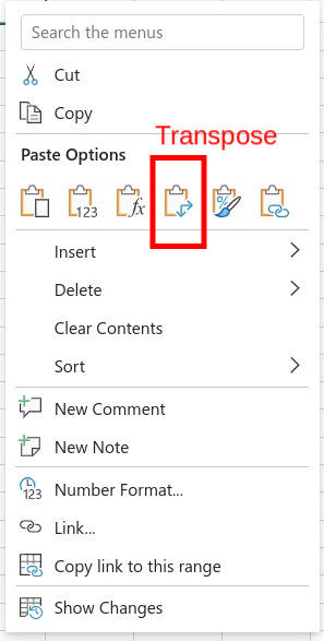
- Your column will now be transferred to a row. Voila!
And you can also use Transpose to do the opposite, that is change a row of data into a column – see below.
Can you imagine how much time this saves rather than copying and pasting each cell into a new row/colum? Just imagine. Or maybe you don’t have to imagine, and like the rest of us, we’ve spent ages copying and pasting data when we could have simply Transposed the data. Anyway, we’re all always learning.
Summary
Give Transpose a go next time you’re using Excel. It’s very simple to do and could save you a lot of pain.
Leave a Reply